Introduction

With classical machine learning, such as Q-learning, a learning agent evolves in a stochastic environment. The agent performs actions and observes their effects on the environment. The learning process is a mix of exploration and exploitation, typically gradually ending in almost entirely exploitation. During exploration, the agent tries at random the available actions, then observes what is happening in the environment. During exploitation, the agent focuses its behaviour on good actions.

Classical machine learning is problematic when a learning agent evolves live in a real stochastic environment such as in cyber-physical security applications. During exploration, the blind random action selection strategy does not work well in all circumstances, especially in non-simulated physical environments. The agent randomly selects a random action without considering the consequences. It does and it observes. The so-called reward may be disastrous and irreversible. This problem can be addressed by augmenting learning agents with “what if I perform this action?” thinking ability. Pearl (2019) proposed extending classical machine learning with causal reasoning. In the proposed three-level hierarchy, this capability corresponds to the second level, called intervention, and can address the “what if?” type of questions. During exploration, with an ability to predict what will happen, a learning agent can limit itself to a subset of cautious actions and exclude the reckless ones.

Cyber-physical Security and “what if?” Reasoning

The ability to predict what will happen when an agent explores a new action finds use in numerous applications, such as in cyber-physical security and the management of the equilibrium between defenders and adversaries. For an adversary, attacking a system implies the execution of multiple actions, such as manipulating signals, impersonating devices and flooding a network with spurious data. For a defender, mitigating such actions also requires the prediction of the system responses, i.e., to anticipate and avoid potential collateral damages. This paradigm has been traditionally used in risk assessment methodologies, including the use of attack simulation tools by Ou et al. (2005), in which the actions conducted by adversaries and defenders are represented as sequences of incremental steps. The last steps of an attack simulation sequence correspond to events that can be detrimental to the system. In this sense, an attack analysis tool can benefit from prediction abilities in two different ways: (i) to proactively anticipate the attack sequences leading to the detrimental events or (ii) to reactively correlate the response plans. Even more, since both (i) and (ii) find their nature in the use of causality, it is possible to automate and transform attack sequences into response plans, which turns out to be much easier and more efficient [Godefroy et al., 2015].

The Quantum Way

Agents with causal reasoning ability need a model of their environment that can be queried to answer, “what if?” questions. Classical modelling tools, such as Bayesian networks, can be used for predictive modelling. Barbeau & Garcia-Alfaro (2022) recently highlighted the advantages that quantum computing can provide in the cyber-physical security landscape, either to an adversary or to a defendant. Moreover, Yang et al. (2022) established quantum foundations for predictive modelling. They highlight the double challenges of predicting accurately while minimizing the required quantum resources, such as memory. They proposed an approach for non-Markovian processes; that is, in environments where the probability of an event does not depend only on the current state. The processes are modeled by random variables. In this article, we push the idea a little further. We develop a quantum predictive modelling approach for environments modelled by unistochastic processes, a subset of Markovian processes, that is, in environments where the probability of an event does depend only on the current state.

An Example

The cat and mouse metaphor captures the essence of a cyber-physical security problem. The mouse, the physical system, must accomplish a goal, under constant threat from the cat, the adversary. Let us consider the example pictured in Figure 1b. Suppose a world comprising a cat, a mouse, and a piece of cheese. The mouse needs the cheese to survive. The cat likes to wander. The mouse needs to effectively create a strategy to reach the cheese while at the same time avoiding being caught by the cat. This is made more complicated by the fact that the cat does not necessarily move in a deterministic fashion.

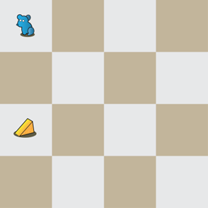
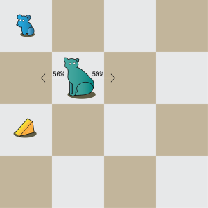
While quite simple, this scenario is closely analogous to many instances of adversarial environments in cyber-physical security. Wherein our defender (the mouse) must dynamically employ various strategies (such as move up, or move down), to accomplish a goal (eating cheese), while at the same time an adversary is probabilistically choosing strategies. Choosing the best actions to take even in this simplified scenario is expensive using classical methods. While at the same time, using classical heuristics to improve performance may have a higher risk of choosing bad actions, which can be fatal.

Quantum Representation

The reader not familiar with quantum computing concepts, notation and circuits is invited to read books authored by Bernhardt (2020), Mannucci and Yanofsky (2008) and Nielsen and Chuang (2010). Our goal is to have an agent that leverages quantum computing to choose sequences of actions effectively and efficiently in environments with antagonistic agents, such as in the cat and mouse example. In our example, a mouse navigates a 2D grid space, attempting to gather cheese and avoid a cat simultaneously. To achieve this efficiency, we use a powerful extension to the quantum Grover’s algorithm that allows for weighted outcomes.

In the standard uses of Grover’s algorithm, a black-box function  f (x) , called the oracle, is assessed. The oracle takes a sequence of bits and returns 1 when x satisfies the function, or 0 when x does not. This can be used for anything from determining factors of a large number to finding an element with a particular property in an unstructured database. Using normal computational methods, when dealing with an input space of n bits with N = 2^n elements, the time complexity for these problems is an expected N / 2. However, by using Grover’s algorithm, we have the significantly improved time complexity of √N, as demonstrated in the sequel.

For our purposes, we use an extension of Grover’s algorithm where instead of returning either 0 or 1, our oracle returns superpositions of 0 and 1 [Mayfield 2016]. The more desirable our input to the oracle function, the higher the probability amplitude of output state 1. With this simple modification to the definition of an oracle, we obtain significantly different behaviour. This extended algorithm has the following property: after completion, more desirable states are more likely to be measured than less desirable states. In our case, we use Grover’s extended algorithm to rank and probabilistically choose good sequences of actions for the mouse.

As this extended algorithm only differs in the definition of an oracle function, it is worth going into some detail about how this oracle function works. Our design is made up of mostly auxiliary qubits – which store information such as the position of the cat and mouse, cumulative reward, whether the mouse has been captured, and more. The actual input qubits of the algorithm represent the action sequence the mouse takes. Note that when designing an oracle for Grover’s algorithm, you need not worry about superpositions of states; if it works for the individual states in the computational basis, it works in general.

We explain in detail the quantum representation of the environment, mouse actions, cat actions and reward. The environment is represented by two quantum state components, an x component and a y component, see Figure 2. For example, |01,10⟩ represents the grid square located at row 01 and column 10. Each state of the environment has two parts. The first half of the qubits represents the x and y position of the cat, and the second half represents the  and  position of the mouse:

A significant advantage of representing the environment as a quantum state is the use of superpositions. For example, one useful aspect of this is that we can represent non-deterministic evolution, since a quantum state can represent multiple classical states simultaneously. The goal of our algorithm is to get a quantum state that when measured has a high probability of giving us a high reward sequence of mouse actions. This sequence of actions is encoded in a binary form as a string of actions, where each action is represented by a few bits and a sequence of actions is represented by an array of actions. After each turn, we update the environment and analyze it. The mouse has four possible moves, move right, up, left, or down. An action sequence is represented as a string of 2m qubits, where m represents the number of actions in the sequence. A given action sequence will have the following quantum representation:

Every action is two qubits. The basis vectors |00⟩,  corresponds to moving right, |01⟩ , to moving up, |10⟩ to moving left, and |11⟩ to moving down.

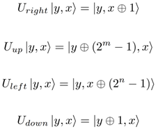
The state of the environment evolves over time in a unitary fashion. We use quantum unitary matrices that correspond to the unistochastic matrices in a Unistochastic Markov Decision Process. The unitary matrices represent the mouse travelling right, up, left, or down. Each of these can be interpreted as a unitary permutation. Let the x dimension be represented with n bits, and the y dimension be represented with m bits. The unitary transformations are as follows:

For the sake of simplicity, let us limit the cat to moving only either left or right. The movements of the cat are determined by a quantum binary string in a uniform superposition. In practice, this means that we model the cat moving either right or left at each timestep with equal probability. Note that the quantum implementation means modelling a cat with multiple possible paths has a relatively negligible impact on time complexity.

The most important element of the environment is to analyze the reward. Following each state change, we take the reward at the grid space the mouse is currently located and add that to a running total. Next, we check to see if the cat and mouse occupy the same space. If that is the case, we consider the mouse dead and set the reward of that action sequence to null. After running through each time step and adding up the reward, we are left with a completed oracle. Then, we run Grover’s algorithm with said oracle as normal. When the resulting quantum state is measured, the probability of measuring a particular sequence of moves is proportional to the reward earned by that sequence of moves. Let r denote a particular reward, 0≤r≤1. The reward bit is initialized to zero. The unitary implementation of a reward function R acting on |state, reward⟩ has the following definition:

Let us consider the cat, mouse and cheese example of Figure 1b. We have a four-by-four grid. Without food, the mouse starves. In this case, we interpret every space without cheese as having a zero reward, and a cheese space to have a unit reward.

Quantum Processing

We discuss the construction of the quantum circuitry implementing the oracle function that is used in conjunction with Grover’s extended algorithm. We model a sequence of actions in an environment with rewards in our oracle. In more specific terms, let |λ⟩ = α |0⟩ + β |1⟩ represent our oracle’s output bit. The oracle function does the following:

●      When a sequence of actions leads to high reward, maximize β.

●      When a sequence of actions leads to low reward, maximize α.

This oracle results in high value action sequences having higher likelihoods.

The circuit in Figure 3 details the quantum processing of a single action using the unitary matrices. Each move corresponds to a unitary matrix U_i. . Where U_i. represents the Markov matrix associated with the move i. We use not (x) gates to ensure that when the qubits correspond to move i, the gate implementing matrix U_i acts on the environment. For this circuit starting with |ψ,ϕ⟩ = |10⟩, we have: |ψ_0,ϕ_0⟩ = |01⟩, |ψ_1,ϕ_1⟩ = |00⟩, |ψ_2,ϕ_2⟩ = |11⟩, |ψ_3,ϕ_3⟩ = |10⟩. This implies that, with input 0b10 in binary or 2 in decimal, the matrix U_2 is activated, while the others are not.

Action sequences follow naturally. They can be arbitrarily long. However, the number of action bits corresponds to exponential computational time complexity, which should be kept in mind. Figure 4 show the quantum circuit for a sequence of k actions |ψ_i⟩ , 1 ≤ i ≤ k where each action is represented with m qubits, and the state |ω⟩ is represented by n bits. Every Action box embeds an instance of the circuit in Figure 3.

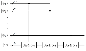
Figure 5 shows the design of the quantum reward circuit. The action |ψ⟩ is represented by m qubits. The state |ω⟩ is represented by n qubits. The reward bit is initialized to |0⟩. The block Action represents an instance of the circuit in Figure. The block represents the quantum gate implementing the reward function.

Grover’s Algorithm

Grover’s algorithm is one of the two most influential quantum algorithms (Shor’s algorithm for factoring being the other). While it was originally designed to search databases, it guarantees a quadratic speedup for various other applications. More specifically, for classical problems that usually take time in O(n) operations, Grover’s Algorithm can solve them in O(√n) operations. This quadratic speedup can also be used in conjunction with other quantum speedups. For our application, we use an extended version of Grover’s algorithm that takes desirability into account.

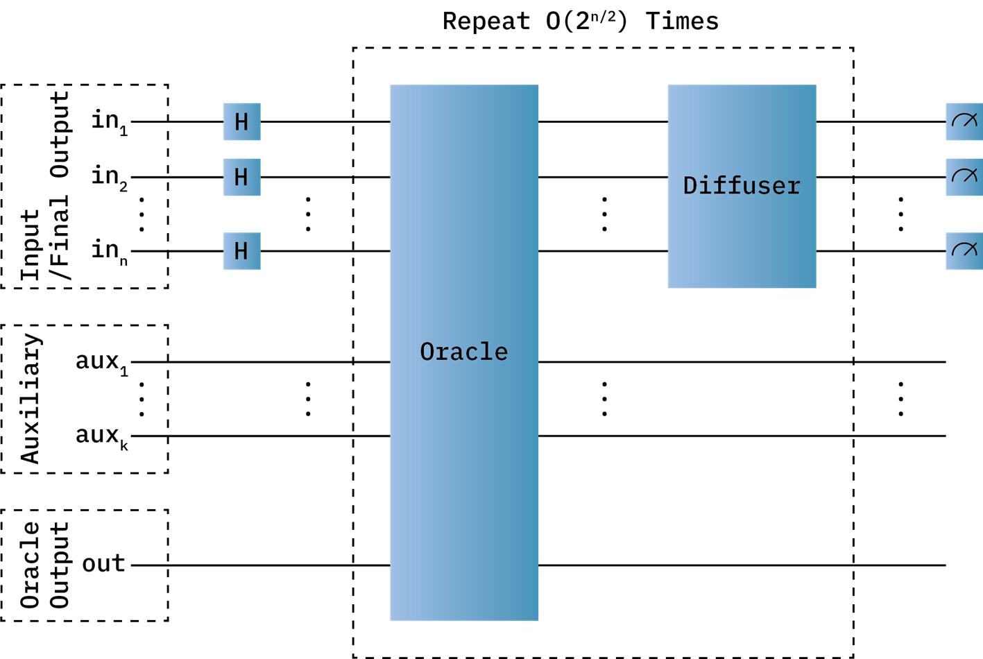
Using Grover’s algorithm quantum circuit design in Figure 6, the quantum process, described in Figures 3, 4 and 5, is run repeatedly. Grover’s algorithm has a few steps. First, the input qubits are initialized to a uniform state using Hadamard (H) gates. These qubits also serve as the final output of Grover’s algorithm. The input/final output qubits represent an action sequence. Then, the Oracle is run on all qubits. The Oracle box is the quantum representation of our function. A diffuser circuit is run on the input bits. The diffuser reflects the uniform state produced with Hadamard gates. It is essential for Grover’s algorithm to function. The process is repeated until a desirable final output is likely. In the worst case, the number of iterations required to get a correct answer is on the order of 2^(n/2). When using Grover’s extended algorithm, we use random numbers of iterations less than 2^(n/2). We run the entire algorithm multiple times until we get a good output. In this example, the auxiliary qubits represent the state, the cat’s sequence of moves, and more. The oracle output bit deals with the quantum output of the oracle function. It stores the quality of each state in a superposition.

Let us consider a four-by-four grid world of Figure 1a consisting of the mouse and cheese only. After three runs of the circuit in Figure 6, we obtain a 45.5% chance of doing the action sequence up-up, wrapping around to the cheese, and a 45.5% chance of doing the action sequence down-down, to the cheese. Let us add a cat to this situation, with a 50/50 chance of moving left/right on each timestep, as is shown in Figure 1b. In this case, after three runs of Grover’s algorithm, we have a 65.4% chance of doing the action sequence up-up, safely avoiding the cat and getting the cheese (avoiding starvation), but a 23.9% chance of taking the risky down-down path to the cheese.

Consider the following scenario, suppose the mouse is not at risk of starvation (e.g., it is not especially hungry), we could bias every zero states to have a reward of 0.5. In theory, this would result in the mouse being less likely to risk going down the path with the cat. However, Grover’s algorithm performs less predictably as more viable solutions exist. This means that our algorithm will not always be applicable and that a certain range of sparsity of rewards is necessary (between 1 action sequence and a quarter of the possible action sequences being valid solutions very roughly constitutes that range). Further research into what kinds of systems pose this problem will be essential to finding where and when to use our algorithm.

Discussion

In our analysis, the space complexity for dealing with this problem with a classical or a quantum approach would be similar. However, the difference in time complexity is significant. First, we acknowledge a few important facts. Our analysis assumes a brute force method for the classical computation since it would most closely relate to our quantum computation. It should also be noted that this methodology could be extended far past games of cat and mouse and even beyond a 2D grid while maintaining these performance benefits. Following that, we should also note that this example is highly deterministic; each action from each agent has only one possible outcome; in our quantum setting, increasing the number of outcomes would have a negligible performance impact, the same cannot be said in the classical case.

Let depth d be the number of turns performed sequentially. Let the number of mouse moves M_m be the number of discrete possible moves the mouse can make per turn, and the number of cat moves M_c be the number of discrete possible moves the cat can make per turn. Then, assuming the classical calculation for cumulative reward is instantaneous, we have the following complexities. For the classical case, we have:

O_c=M_c^d⋅M_m^d

While on the other hand, the quantum case has a clear advantage with time complexity (for both factors):

O_q=d(M_m+M_c )⋅M_m^(d/2)

This is a significant improvement on multiple fronts. The first square roots the right factor, and the second brings down the exponent d. However, it is worth noting that the quantum algorithm yields probabilistic results and would likely need a constant factor to compensate for repeatedly running the algorithm to increase the likelihood of measuring good action sequences. The code for this example is available on a Github page.

References

Barbeau, M., & Garcia-Alfaro, J. (2022). Cyber-physical defence in the quantum Era. Scientific reports, 12(1), 1-11.

Bernhardt, C. (2020). Quantum Computing for Everyone. Royaume-Uni: MIT Press.

Godefroy, E., Totel, E., Hurfin, M., & Majorczyk, F. (2015). Assessment of an Automatic Correlation Rules Generator. International Conference on Information Systems Security (ICISS 2015), pages 207-224.

Mayfield, L. (2016). Quantum Searching: A survey of Grover’s Algorithm and its Descendants. Available online: https://citeseerx.ist.psu.edu/viewdoc/download?doi=10.1.1.117.6361&rep=rep1&type=pdf

 Ou, X., Govindavajhala, S., & Appel, A. (2005).  MulVAL: A logic-based network security analyzer. In: 14th USENIX Security Symposium, Baltimore, Maryland, USA.

Pearl, J. (2019). The seven tools of causal inference, with reflections on machine learning. Communications of the ACM, 62(3), 54-60.

Mannucci, M. A., Yanofsky, N. S. (2008). Quantum Computing for Computer Scientists. États-Unis: Cambridge University Press.

Nielsen, M. A., Chuang, I. L. (2010). Quantum Computation and Quantum Information: 10th Anniversary Edition. Royaume-Uni: Cambridge University Press.

Yang, C., Garner, A., Liu, F., Tischler, N., Thompson, J., Yung, M. H., … & Dahlsten, O. (2021). Provable superior accuracy in machine-learned quantum models. arXiv preprint arXiv:2105.14434.